
This short tutorial describes how to setup a quantitative phase analysis trough the dedicated wizard. Please note that this procedure is supported from ReX v. 0.9.3; the manual analysis described here is still available but not really recommended, even though it may still be worth to have a look at it at least once.
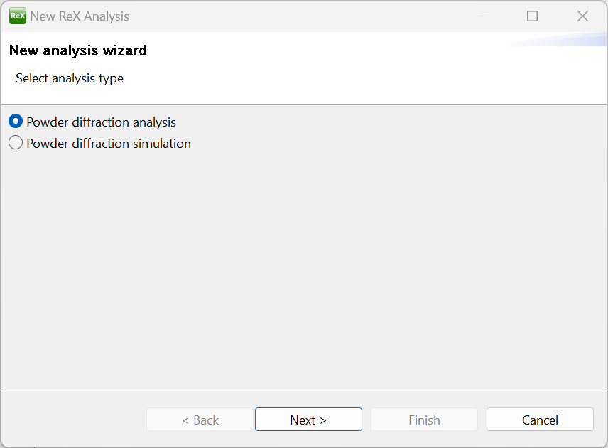
After loading ReX, a welcome screen is displayed with several options; choose the “New analysis wizard” button to start the analysis setup. If no welcome screen is displayed, click “New->New Analysis” from the File menu. In the first wizard panel, select the “Powder Diffraction Analysis” and click “Next >”.
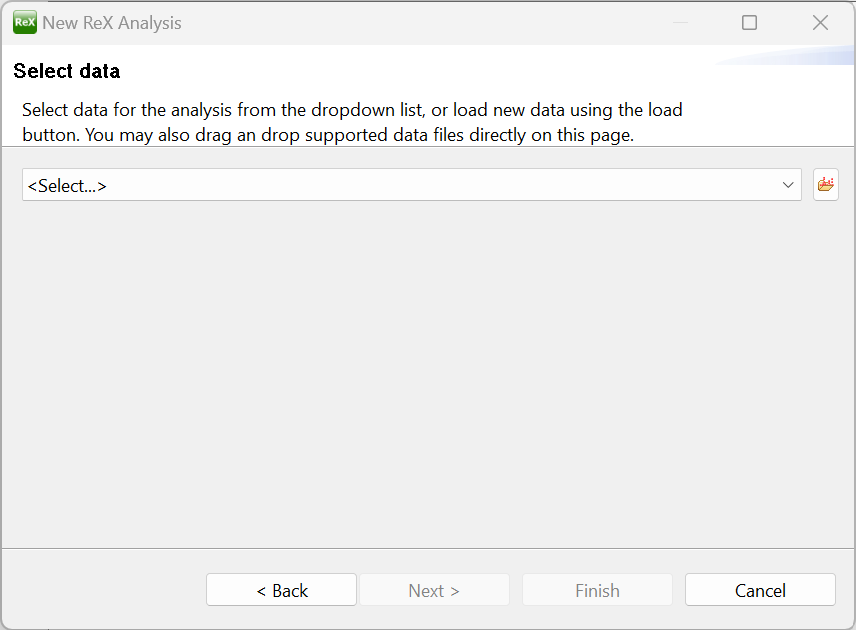
After that, the data setup panel will be shown; as described in the wizard page, powder diffraction data can be loaded (if not already present in the project) by clicking the load button  or by simply dropping supported file formats in the middle of the wizard panel. For this tutorial we are going to use diffraction data coming from the IUCR CPD Round Robin on Quantitative Phase Analysis; the data itself, as well as the instrument calibration and reference CIF files can be found in the cpd_qa folder of the ReX examples archive.
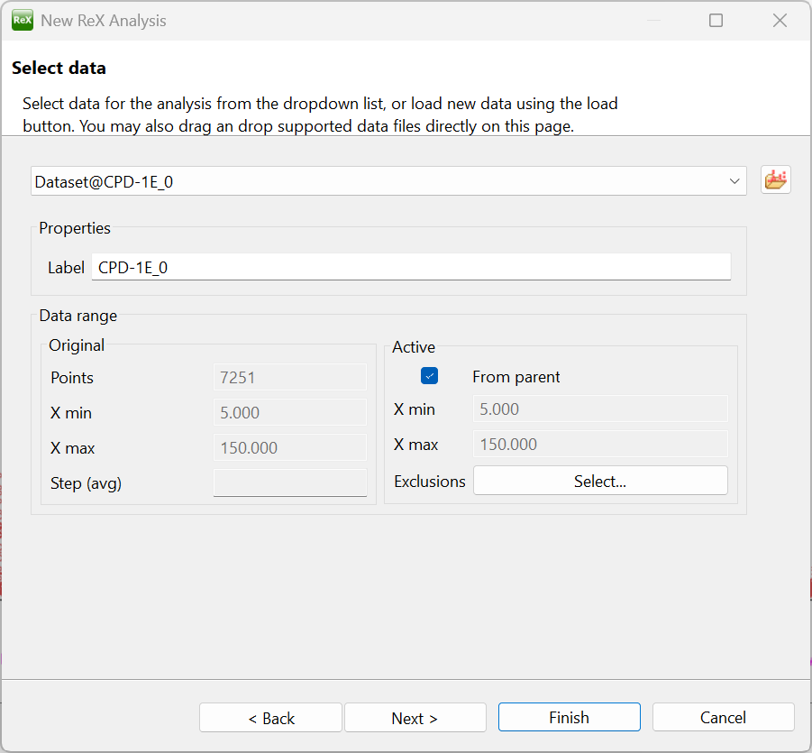
Select the CPD-1E.xy file from the cpd_qa folder and confirm the dialog to load the pattern in the default dataset; the data should be displayed in the main Dataset plot window. Leave the active data range unchanged for now; click next.
The instrument definition panel will show up with a default instrument preloaded.
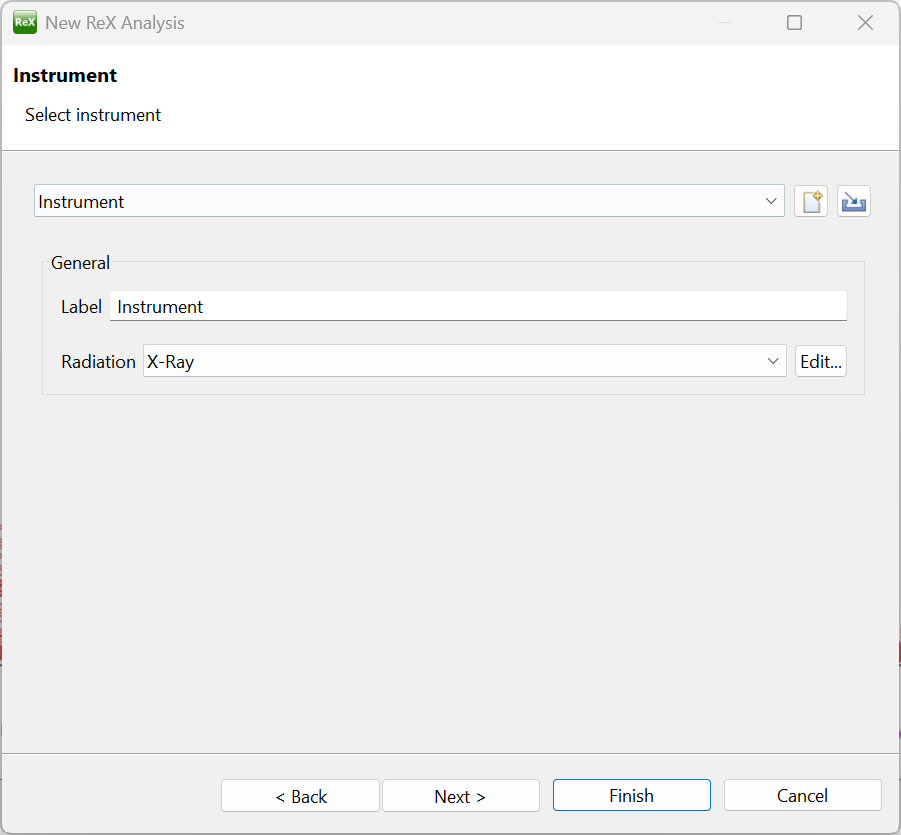
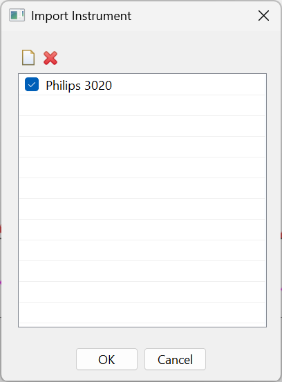
To correclty model the peak broadening though, we need the specific calibration for the instrument used in the CPD data acquisition; to do so, click the import button  located next to the instrument combo and load the cpd-calibration.rxp project file. A dialog will appear to select the instrument configuration; make sure to click the Philips 3020 checkbox and then click OK to associate the instrument with the current dataset.
After clicking “Next” on the bottom of the wizard page, the sample panel will be displayed. Here, the sample model can be defined by loading the corresponding crystallographic phases.
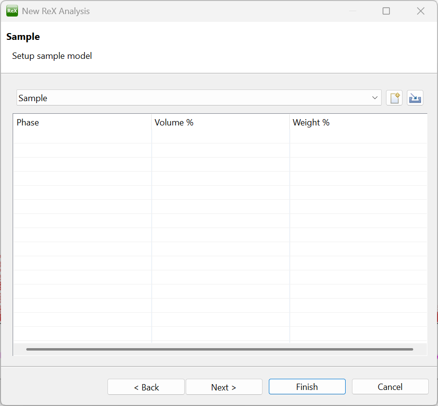
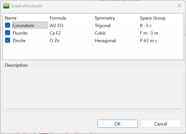
In our case, we need to load the three crystal phases contained in the CPD-E sample (which are already known from the Round Robin sample description), namely Al2O3, CaF2 and ZnO. To do so, drag the three corresponding CIF files located in the cpd_qa folder and drop them on the table. A confirmation dialog will appear; make sure to select all three phases and click OK, then Next on the bottom of the wizard.
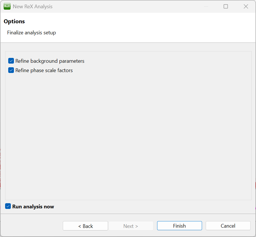
The final wizard panel will appear; make sure the “Refine background parameters”, “Refine phase scale factors” and “Run analysis now” are checked and then click Finish.
The analysis is then carried out by refining all the background and phase scale parameters; the obtained fit is displayed in the Dataset plot window.
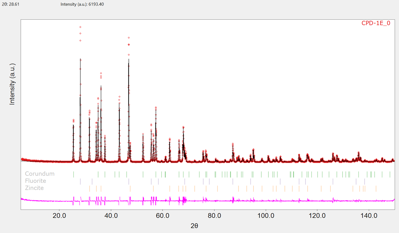
By default, the modeled diffraction pattern is displayed as a continuous black line, whereas the experimental points are represented with red marks; you may configure colors and style of different plot elements selecting the Options command  in the drop-down menu located in the top right corner of the Dataset plot view:
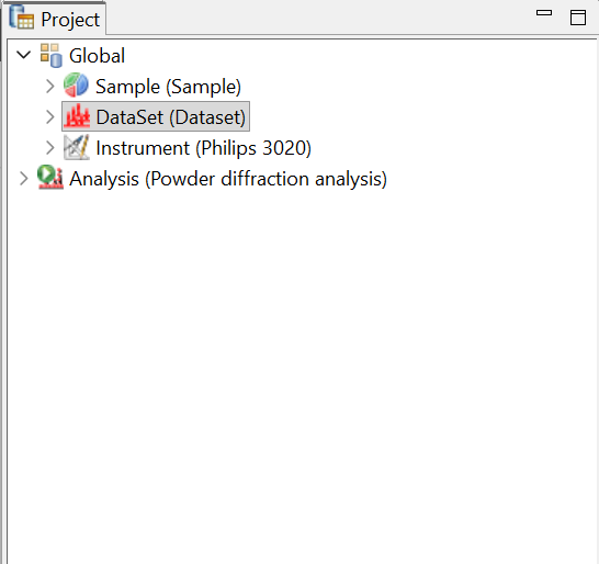
Before going on with the refinement, it is worth spending some time optimizing the fit display. First of all, we are going to slightly reduce the active computation range of the pattern. Make sure the Properties view is visible, and select the Dataset object under the Global node in the Project tree view:
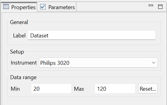
The active pattern data interval is displayed in the Properties view; in the “Used” data subpanel, type 20 and 120 for the 2-Theta min and max values, respectively. The dataset plot gets updated accordingly.
To better visualize the details in the high angle region of the pattern, it is usually convenient to change the scale of the y plot axis to display the squared roots of the intensity counts. To do so, select the “Y axis scale” menu  located on the top of the Dataset plot view and choose the “square root” option; the plot view is updated accordingly. After that, it may be also convenient to display the single phase contributions to the modeled diffraction pattern in addition to the total calculated sum. To do so, select the Plot view settings drop-down menu
 (right of the Y scale command just selected) and select the “Show phases plot”
 option.
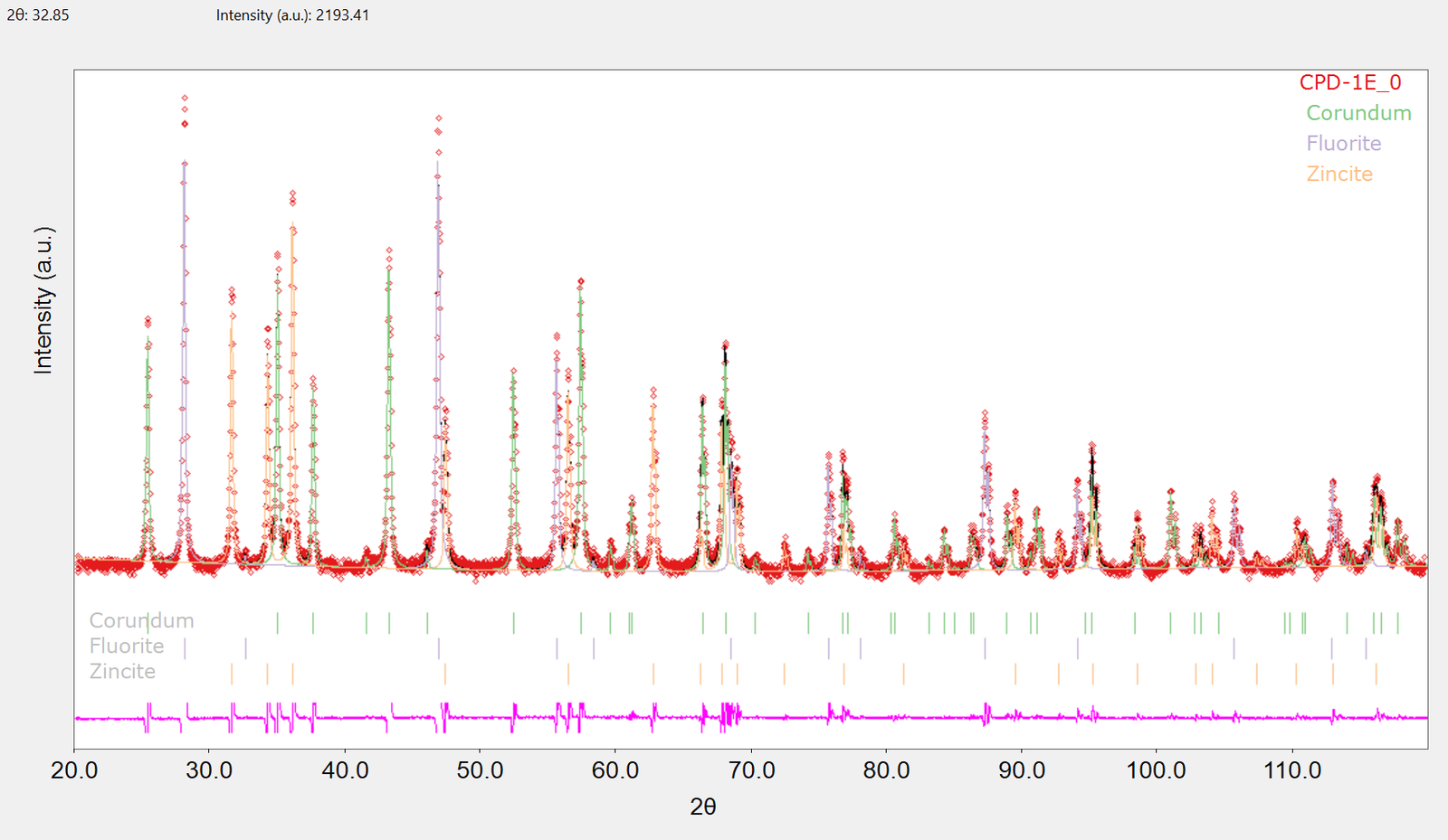
Next, we are going to examine the fit a little bit deeper. By zooming in (drag rectangle with the left mouse button) we can see that there is a small – and more or less systematic – shift between calculated and experimental data, as shown as an example in the figure below (30°-40° 2-Theta).
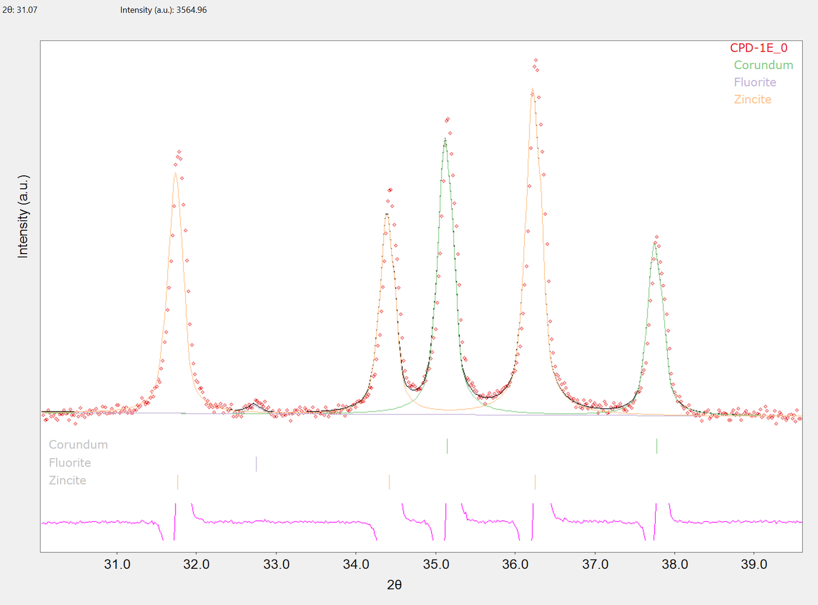
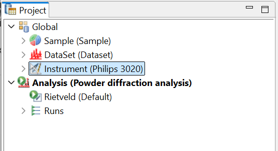
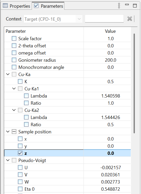
This kind of misalignment can have different origins, the most common being instrumental errors or mismatched lattice parameters; in our case, there are strong hints that z sample displacement is the most likely source of the error. This can be taken into account by refining the sample z position; thus, we need to enable the refinement of the corresponding parameter in the model tree. To do so, make sure the Parameters view is visible and select the “Philips 3020” instrument under the global node near the top of the Project tree; the corresponding model definition will appear in the context-sensitive Parameter tree. Here, enable the refinement of the z sample position parameter by clicking on the corresponding checkbox.
After that, we can manually run the analysis again by clicking the  button on the main toolbar or choosing the “Run analysis” command from the Analysis menu in the application main menu. After a few iterations, the final fit is shown with visibly better agreement between experimental and calculated data; from the log view (by default, located just below the Dataset plot view) we can notice that the Rwp value significantly improved as well. The latter, as well as phases weight fractions and background parameter values, are reported in the Results view (located again just below the plot view); from here, they can be exported in a text file ‘by clicking the corresponding button
 on the top right corner of the Results view itself.